Variance: regression, clustering, residual and variance – Liyun Chen ’11

Liyun ChenLiyun Chen ’11 (Economics) is Senior Analyst for Data Science at eBay. She recently moved from the company’s offices in Shanghai, China to its headquarters in San Jose, California. The following post originally appeared on her economics blog in English and in Chinese. Follow her on Twitter @cloudlychen


Variance is an interesting word. When we use it in statistics, it is defined as the “deviation from the center”, which corresponds to the formula  \sum (x- \bar{x})^2 / (n-1), or in the matrix form Var(X) = E(X^2)- E(X)^2=X'X/N-(X'1/N)^2(1 is a column vector with N*1 ones). From its definition it is the second (order) central moment, i.e. sum of the squared distance to the central. It measures how much the distribution deviates from its center — the larger the sparser; the smaller the denser. This is how it works in the 1-dimension world. Many of you should be familiar with these.

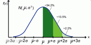
Variance has a close relative called standard deviation, which is essentially the square root of variance, denoted by \sigma// . There is also something called the six-sigma theory– which comes from the 6-sigma coverage of a normal distribution.

79f0f736afc37931c22b82ecebc4b74542a911b7.jpg

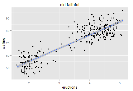
Okay, enough on the single dimension case. Let’s look at two dimensions then. Usually we can visualize the two dimension world with a scatter plot. Here is a famous one — old faithful.
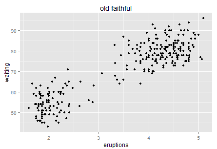
2014-12-27 23_41_46-Plot ZoomOld faithful is a “cone geyser located in Wyoming, in Yellowstone National Park in the United States (wiki)…It is one of the most predictable geographical features on Earth, erupting almost every 91 minutes.” We can see there are about two hundreds points in this plot. It is a very interesting graph that can tell you much about Variance.

Here is the intuition. Try to use natural language (rather than statistical or mathematical tones) to describe this chart, for example when you take your 6 year old kid to the Yellowstone and he is waiting for next eruption. What would you tell him if you have this data set? Perhaps “I bet the longer you wait, the longer next eruption lasts. Let’s count the time!”. Then the kid has a glance on your chart and say “No. It tells us that if we wait for more than one hour (70 minutes) then we will see a longer eruption in the next (4-5 minutes)”. Which way is more accurate?

Okay… stop playing with kids. We now consider the scientific way. Frankly, which model will give us a smaller variance after processing?

Well, always Regression first. Such a strong positive relationship, right? ( no causality…. just correlation)

2014-12-27 23_51_53-Plot Zoom

Now we obtain a significantly positive line though R-square from the linear model is only 81% (could it be better fitted?). Let’s look at the residuals.
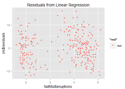
2014-12-27 23_59_10-Plot ZoomIt looks like that the residuals are sparsely distributed…(the ideal residual is white noise which carries no information). In this residual chart we can roughly identify two clusters — so why don’t we try clustering?

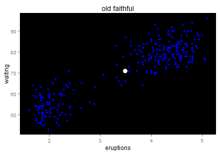
Before running any program, let’s have a quick review the foundations of the K-means algorithm. In a 2-D world, we define the center as (\bar{x}, \bar{y}) // , then the 2-D variance is the sum of squares of each pint going to the center.
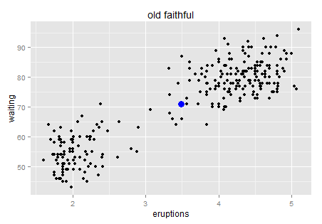
2014-12-28 00_09_03-Plot ZoomThe blue point is the center. No need to worry about the outlier’s impact on the mean too much…it looks good for now. Wait… doesn’t it feel like the starry sky at night? Just a quick trick and I promise I will go back to the key point.


2014-12-28 00_25_06-Plot Zoom

For a linear regression model, we look at the sum of squared residuals – the smaller the better fit is. For clustering methods, we can still look at such measurement: sum of squared distance to the center within each cluster. K-means is calculated by numerical iterations and its goal is to minimize such second central moment (refer to its loss function). We can try to cluster these stars to two galaxies here.
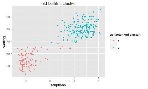
2014-12-28 00_32_00-Plot ZoomAfter clustering, we can calculate the residuals similarly – distance to the central (represents each cluster’s position). Then the residual point.
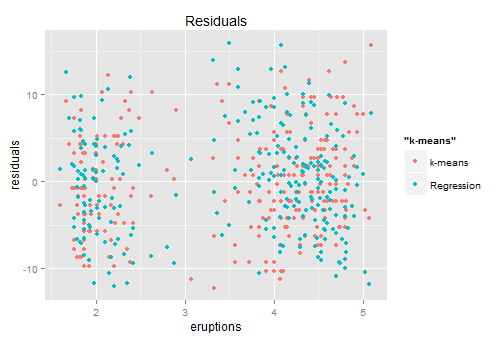
 

2014-12-28 00_51_13-Plot ZoomRed ones are from K-means which the blue ones come from the previous regression. Looks similar right?… so back to the conversation with the kid — both of you are right with about 80% accuracy.

Shall we do the regression again for each cluster?
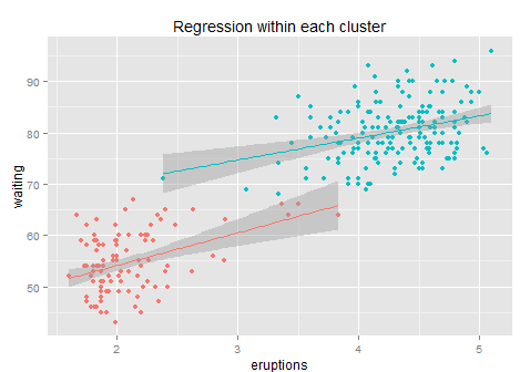
2014-12-28 01_01_20-Plot ZoomNot many improvements. After clustering + regression the R-square increases to 84% (+3 points). This is because within each cluster it is hard to find any linear pattern of the residuals, and the regression line’s slope drops from 10 to 6 and 4 respectively, while each sub-regression only delivers an R-square less than 10%… so not much information after clustering. Anyway, it is better than a simple regression for sure. (the reason why we use k-means rather than some simple rules like x>3.5 is that k-means gives the optimized clustering results based on its loss function).

Here is another question: why do not we cluster to 3 or 5? It’s more about overfitting… only 200 points here. If the sample size is big then we can try more clusters.

Fair enough. Of course statisticians won’t be satisfied with these findings. The residual chart indicates an important information that the distribution of the residuals is not a standard normal distribution (not white noise). They call it heteroscedasticity. There are many forms of heteroscedasticity. The simplest one is residual increases when x increases. Other cases are in the following figure.
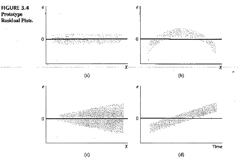
p109figureThe existence of heteroscedasticity makes our model (which is based on the training data set) less efficient. I’d like to say that statistical modelling is the process that we fight with residuals’ distribution — if we can diagnose any pattern then there is a way to improve the model. The econometricians prefer to name the residuals “rubbish bin” — however it is also a gold mine in some sense. Data is a limited resource… wasting is luxurious.

Some additional notes…

Residuals and the model: as long as the model is predictive, then residuals exist, regardless of the model’s type, either a tree or linear or whatever. Residual is just the true Y minus the prediction of Y (based on training data set).

Residuals and loss function: for ordinary least squares, if you solve it in the numerical way then it iterates by the SSR (sum of squared residuals) loss function (equals to the variance of residuals). In fact many machine learning algorithms relay on a similar loss function setting — either first order or higher order moments of residuals. From this perspective statistical modelling is always fighting with residuals. This differs from what the econometricians do so there was a huge debate on the trade off between consistency and efficiency. Fundamentally different believes of modelling.

Residuals, Frequentists and Bayesians: In the above paragraphs I mainly followed the Frequentist’s language. There was nothing on posterior… From my understanding many items there would be mathematically equivalent to the Bayesian’s frameworks so it should not matter. I will mention some Bayesian ideas in the following bullets so go as you wish.

Residuals, heteroscedasticity and robust standard error: We love and hate heteroscedasticity at the same time. It tells us that our model is not perfect while there is a chance to make some improvements. Last century people tried to offset heteroscedasticity’s impact by introducing the robust standard error concept — Heteroscedasticity-consistent standard errors, e.g. Eicker–Huber–White. Eicker–Huber–White changes the common sandwich matrix (bread and meat) we use for the significant test (you may play with it using the sandwich() package in R). Although Eicker–Huber–White contributes to the variance estimation by re-weighing with estimated residuals, this approach does not try to identify any patterns from the residuals. Thus there are methods like Generalized least square (GLS) and Feasible generalized least square (FGLS) that try to use a linear pattern to reduce the variance. Another interesting idea is clustered robust standard error which allows heterogeneity among clusters but constant variance within each cluster. This approach only works when the number of groups approaches infinite asymptotically. (otherwise you will be getting stupid numbers like me!)

Residuals and reduction of dimensions: generally speaking the more relevant co-variates introduced to the model the less the noise is; while there is also a trade-off towards overfitting. That is why we need to reduce the dimensions (e.g. via regularization). Moreover, it is not necessary that we want to make a prediction every time; sometimes we may want to filter out the significant features — a sort of maximizing the information we could get from a model (e.g. AIC or BIC or attenuation speed which increasing the punishment in regularization). In addition regularization is not necessarily linked to train-validation… not the same goal.

Residuals and experimentation data analysis: heteroscedasticity will not influence the consistency of Average Treatment Effect estimation in an experimentation analysis. The consistency originates from randomization. However people are still eager to learn more beyond a simple test-control comparison, especially when the treated individuals are very heterogenous; they look for heterogenous treatment effect. Quantile regression may help in some case if there is a strong covariate observed…but what could we do when there are thoudsands of dimensions? Reduce the dimension first?

Well, the first reaction to “heterogeneous” should be variance…right? otherwise how could we quantify heterogeneity? There is also a bundle of papers that try to see whether we would be able to find more information for treatment effects rather than simple ATE. This one for instance:

Ding, P., Feller, A., and Miratrix, L. W. (2015+). Randomization Inference for Treatment Effect Variation. http://t.cn/RzTsAnl

View full code in the original post on Ms. Chen’s blog

The Mission: Human Capital and the Persistence of Fortune – Job Market Paper

Job market paper Felipe Valencia ’15 (GPEFM – UPF and Barcelona GSE)

Felipe ValenciaThe following job market paper summary was contributed by Felipe Valencia (GPEFM – UPF and Barcelona GSE).

**Update: This paper has now been published in the Quarterly Journal of Economics and featured in the The Washington Post!**


The importance of history in economic development is well-established (Nunn 2009; Spolaore and Wacziarg 2013), but less is known about the specific channels of transmission which drive this persistence in outcomes. Dell (2010) stresses the negative effect of the mita in Latin America, and Nunn and Wantchekon (2011) document the adverse impact of African slavery through decreased trust. But did other colonial arrangements lead to positive outcomes in the long run?

I address this question in my Job Market Paper by analyzing the long-term economic consequences of European missionary activity in South America. I focus on missions founded by the Jesuit Order in the Guarani lands during the seventeenth and eighteenth centuries, in modern-day Argentina, Brazil and Paraguay. This case is unique in that Jesuits were expelled from the Americas in 1767 –following European “Great Power” politics— precluding any continuation effect. While religious conversion was the official aim of the missions, they also increased human capital formation by schooling children and training adults in various crafts. My research question is whether such a one-off historical human capital intervention can have long-lasting effects.

photo
The author at the site of one of the Jesuit missions on Guarani lands in South America.

Setup

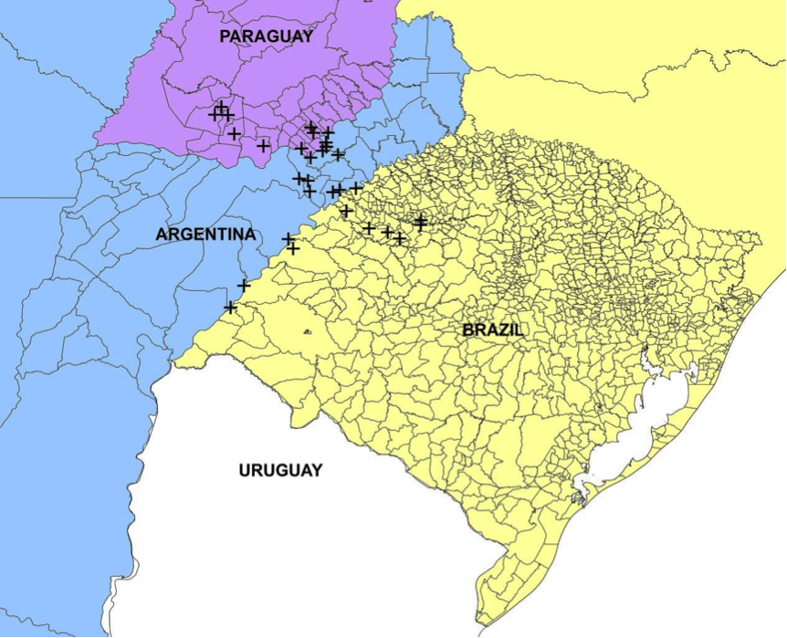
To disentangle the national institutional effects from the human capital shock the missions supplied, I use within country variation in missionary activity in three different countries:

fig1_valencia
Note: The map shows the exact location of the Guarani Jesuit Missions (black crosses) with district level boundaries for Argentina, Brazil and Paraguay.


The area under consideration was populated by a single semi-nomadic indigenous tribe, so I can abstract from the direct effects of different pre-colonial tribes (Maloney and Valencia 2012; Michalopoulos and Papaioannou, 2013). The Guarani area also has similar geographic and weather characteristics, though I control for these variables in the estimation.

Key Findings

Using municipal level data for five states (Corrientes and Misiones in Argentina, Rio Grande do Sul in Brazil, and Itapúa and Misiones in Paraguay), I find substantial positive effects of Jesuit missions on human capital and income, 250 years after the missionaries were expelled. In municipalities where Jesuits carried out their apostolic efforts, median years of schooling and literacy levels remain higher by 10-15%. These differences in educational attainment have also translated into higher modern per capita incomes of nearly 10%. I then analyze potential cultural mechanisms that can drive the results. To do so I conduct a household survey and lab-in-the-field experiments in Southern Paraguay. I find that respondents in missionary areas have higher non-cognitive abilities and exhibit more pro-social behavior.

Endogeneity

Even though I use country and state-fixed effects as well as weather and geographic controls, Jesuit missionaries might have chosen favorable locations beyond such observable factors. Hence the positive effects might be due to this initial choice and not to the missionary treatment per se.

To address the potential endogeneity of missionary placement, I conduct two empirical tests. The first one is a placebo that looks at missions that were initially founded by the Jesuits but were abandoned early on (before 1659). I can thereby compare places that were initially picked by missionaries with those that actually received the missionary treatment. I find no effect for such “placebo” missions, which suggests that what mattered in the long run is what the missionaries did and not where they first settled.

Second, I conduct a comparison with the neighboring Guarani Franciscan Missions. The comparison is relevant as both orders wanted to convert souls to Christianity, but Jesuits emphasized education and technical training in their conversion. Contrary to the Jesuit case, I find no positive long-term impact on either education or income for Franciscan Guarani Missions. This suggests that the income differences I estimate are likely to be driven by the human capital gains the Jesuits provided.

In addition, I employ an IV strategy, where I use as instruments the distance from early exploration routes and distance to Asuncion. Distance from the exploration routes of Mendoza (1535-1537) and Cabeza de Vaca (1541-1542) serves as a proxy for the isolation of the Jesuit missions (in the spirit of Duranton et al. 2014). Asuncion, in turn, served as a base for missionary exploration during the foundational period, but became less relevant for Rio Grande do Sul after the Treaty of Madrid (1750) transferred this territory to Portuguese hands. For this reason and to avoid the direct capital –and Spanish Empire—effects, I use this variable only for the Brazilian subsample of my data (as in Becker and Woessmann 2009; Dittmar 2011). The first-stage results are strongly significant throughout (with F-statistics well above 10), and the second-stage coefficients for literacy and income retain their sign and significance –appearing slightly larger—in the IV specifications.

Extensions and Mechanisms

To complete the empirical analysis, I examine cultural outcomes and specific mechanisms that can sustain the transmission of human capital from the missionary period to the present. I find that respondents in missionary areas possess superior non-cognitive abilities, as proxied by higher “Locus of Control” scores (Heckman et al., 2006). Using standard experiments from the behavioral literature, I find that respondents in missionary areas exhibit greater altruism, more positive reciprocity, less risk seeking and more honest behavior. I use priming techniques to further investigate whether these effects are the result of greater religiosity –which appears not to be the case.

In terms of mechanisms, my results indicate that municipalities closer to historic missions have changed the sectoral composition of employment, moving away from agriculture and towards manufacturing and services (consistent with Botticini and Eckstein, 2012). In particular, I document that these places still produce more handicrafts such as embroidery, a skill introduced by the Jesuits. People closer to former Jesuit missions also seem to participate more in the labor force and work more hours, consistent with Weber (1978). I also find that indigenous knowledge —of traditional medicine and myths—was transmitted more from generation to generation in the Jesuit areas. Unsurprisingly, given their acquired skills, I find that indigenous inhabitants from missionary areas were differentially assimilated into colonial and modern societies. Additional robustness tests suggest that the results are not driven by migration, urbanization or tourism.


Follow Felipe on Twitter

Young and under pressure – Europe is risking a lost generation

The following post by Olga Tschekassin ’13 (Master in International Trade, Finance and Development) has been previously published by the World Economic Forum and Bruegel

Ms. Tschekassin is Research Assistant at Bruegel in Brussels, Belgium. Follow her on Twitter @OlgaTschekassin


Since the beginning of the global financial crisis, social conditions have deteriorated in many European countries. The youth in particular have been affected by soaring unemployment rates that created an outcry for changes in labour market policies for the young in Europe. Following this development, the Council of Europe signed a resolution in 2012 acknowledging the importance of this issue and asking for implementation of youth friendly policies in the Member States. Yet, almost 5.6 million young people were unemployed in 2013 in the European Union (EU) – in nine EU countries the youth unemployment rate more than doubled since the beginning of the crisis.

Today I want to draw your attention to two more indicators reflecting the social situation of the young generation: the percentage of children living in jobless households and the percentage of young people that are neither in employment nor education nor training.

Children in jobless households

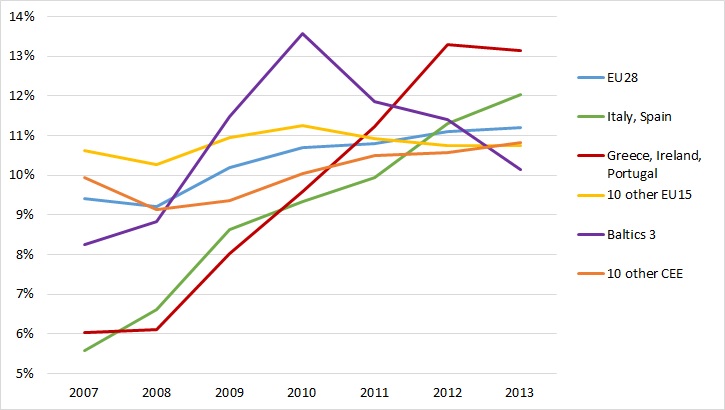
The indicator Children in jobless households measures the share of 0-17 year olds as a share of the total population in this age group, who are living in a household where no member is in employment, i.e. all members are either unemployed or inactive (Figure 1).

Figure 1: Children in jobless households

Source: Eurostat and Bruegel calculations. Country groups: 10 other EU15: Austria, Belgium, Denmark, Finland, France, Germany, Luxembourg, Netherlands, Sweden and United Kingdom; Baltics 3: Latvia, Lithuania, Estonia; 10 other CEE refers to the 10 member states that joined in the last decade, excluding the Baltics: Bulgaria Czech Republic, Croatia, Hungary, Poland, Romania, Slovenia, Slovakia, Cyprus and Malta; Sweden: data for 2007 and 2008 is not available, the indicator is therefore assumed to evolve in line with the other 9 EU15 countries. Such approximation has only a marginal impact on the aggregate of the other EU15 countries, because children in jobless HHs in Sweden represented only 3% of the country group in 2009. Countries in groupings are weighted by population.

In the EU28 countries this share rose only slightly over the past years to 11.2%. It is striking, however, that the ratio of children living in households where no one works more than doubled in the euro-area programme countries (Greece, Ireland, Portugal) as well as in Italy and Spain to 13% and 12%, respectively. And even more shocking – while the share stabilized in the programme countries, in Italy and Spain it is still sharply increasing. In Ireland in 2013 more than one in every six children lived in a household where no one worked. This is indeed an alarming development. Only the Baltics, which experienced a very deep recession among the first countries hit by the crisis, are reporting a sizable turning point in the statistic in 2010 and the share is presently continuing to decline. The numbers are, however, still well above pre-crisis levels.

A high share of children living in jobless households is not only problematic at the moment but can also have negative consequences for the young people’s future since it often means that a child may not only have a precarious income situation in a certain time period, but also that the household cannot make an adequate investment in quality education and training (see a paper on this issue written for the ECOFIN Council by Darvas and Wolff here). Therefore a child’s opportunities to participate in the labour market in the future are likely to be adversely affected. Moreover, as I discussed in a blog earlier this year, children under 18 years are more affected by absolute poverty than any other group in the EU and the generational divide is widening further.

Not in Education, Employment or Training (NEET)

The financial situation of young people between 18 and 24 years old who finished their education is less dependent on their parents income because they usually enter the labour market and generate their own income. Therefore we are going to have a closer look on their work situation, i.e. how many young people have difficulties participating in the labour market.

Figure 2:  Not in Education, Employment or Training
Figure 2: Not in Education, Employment or Training

Source: Eurostat and Bruegel calculations. Country groups as in previous chart

The NEET indicator measures the proportion of young people aged 18-24 years which are not in employment, education or training as a percentage of total population in the respective age group. We can see in Figure 2 that the situation among EU28 countries stabilized over the last four years. The good news is that for the first time since 2007 we see a decline in the rate in the euro-area programme countries in 2013. This decline is, however, mostly driven by Ireland with an unchanged situation in Greece and Portugal. Also, in the Baltics the ratio is on a downward trend. More worrying, however, is the situation in Italy and Spain. Among all EU28 countries, the young generation in Italy with 22.2% of all young people being without any employment, education or training, is disproportionately hit by the deterioration in the labour market. Every fifth young person between 18 and 24 is struggling to escape the exclusion trap. Europe and especially Italy is risking a lost generation more than ever.

Labour market policies for young people should therefore stand very high on the national agendas of Member States. The regulations introduced in summer 2013 into the Italian labour market reform which are setting economic incentives for employers to hire young people build an important step towards more labour market integration of the youth in Europe. Their effects are yet to be observed in the employment statistics in the coming years in Italy. More action on the national and European level is needed to improve the situation of the young.

Heterogeneous Inputs, Human Resource Management and Productivity Spillovers: What Do Poultry Farm Workers Have to Say? – Job Market Paper

authorThe following job market paper summary was contributed by Francesco Amodio (Economics ’10 and GPEFM). Francesco is a job market candidate at UPF. He will be available for interviews at the SAEe (Palma de Mallorca, December 11-13) and ASSA (Boston, January 3-5) meetings.

Management matters. Differences in management practices can explain a considerable amount of variation in firms’ productivity and performance, both across and within sectors and countries (Bloom and Van Reenen 2007, 2010, 2011). Several studies have shown how human resource management and incentive schemes may affect overall productivity by making the effort choices of coworkers interdependent (Bandiera, Barankay and Rasul 2005, 2007, 2009). In more complex settings, however, workforce management features may interact with production arrangements and jointly determine the overall result of the organization. Understanding the nature of this interplay is of primary importance in the adoption and implementation of productivity-enhancing management practices.

In my job market paper, coauthored with Miguel A. Martinez-Carrasco, we shed light on these issues by focusing on settings where workers produce output by combining their own effort with inputs of heterogeneous quality. This is a common feature of workplaces around the world. For instance, in Bangladeshi garment factories, the characteristics of raw textiles used as inputs affect the productivity of workers. Similarly, the purity level of chemicals affects the productivity of researchers in biological research labs.

Now, suppose we pick a worker and endow her with higher quality inputs, thus increasing her productivity. What happens to the productivity of coworkers around her? Do they exert more effort, or do they shirk? How do human resource management features shape their response?

The setting

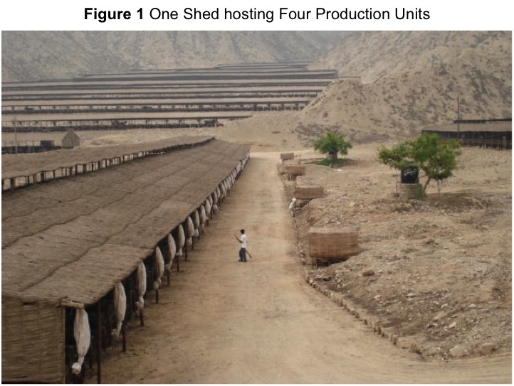
In order to answer these questions, we collected data from an egg production plant in Peru. Production is carried out in production units located one next to the other in several sheds. In each production unit, a single worker is assigned as input a batch of laying hens. Workers’ main tasks are to feed the hens, to maintain and clean the facilities, and to collect the eggs. The characteristics of the hens and worker’s effort jointly determine productivity, as measured by the daily number of collected eggs. Figure 1 shows the picture of one shed hosting four production units. Notice how workers in neighboring production units can easily interact and observe each other.

figure

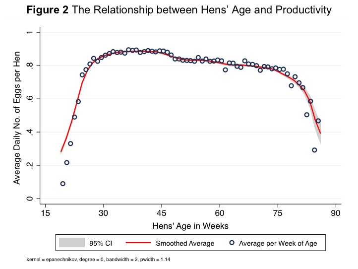
The specific features and logistics of this setting generate the quasi-experiment we need in order to answer the questions of interest. All hens within a given batch have very similar characteristics. When reaching their productive age, they are moved to one production unit and assigned to the corresponding single worker who operates the unit. After approximately 16 months, they reach the end of their productive age and are discarded altogether. The age of hens in the batch exogenously shifts productivity. Indeed, Figure 2 shows the reversed U-shaped relationship that exists between hens’ age and productivity. Perhaps more importantly, the timing of batch replacement varies across production units, generating quasi-random variation in the age of hens assigned to workers.1 We can thus exploit these differences to credibly identify the causal effect of an increase in coworkers’ productivity – as exogenously shifted by coworkers’ hens age – on own productivity, conditional on own hens’ age.

figure

Main Results

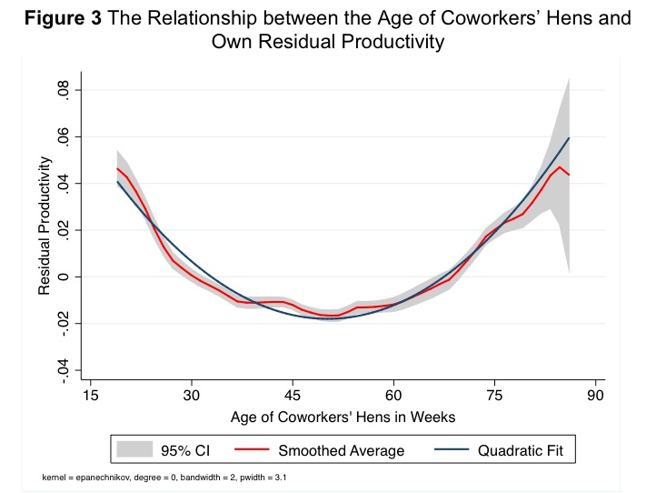
We find evidence of negative productivity spillovers. The same worker, handling hens of the same age, is significantly less productive when coworkers in neighboring production units are more productive, with variation in the latter being induced by changes in the age of their own hens. This finding is pictured in Figure 3, which shows that a U-shaped relationship exists between own productivity and coworkers’ hens age. In other words, workers exert less effort and decrease their productivity when coworkers are assigned higher quality inputs.

figure

We also find similar negative effects on output quality, as measured by the fraction of broken and dirty eggs collected over the total number of eggs. Furthermore, we find no effect of an increase in the productivity of coworkers located in non-neighboring production units or in different sheds, suggesting that workers only respond to observed changes in coworkers’ productivity.

The role of HR

Why do workers exert less effort when coworkers’ productivity increases? Our hypothesis is that the way the management processes information on workers’ productivity in evaluating them and taking employment termination decisions generates free ride issues among coworkers. When observed productivity is only a noisy signal of workers’ exerted effort, the management combines available signals and best guesses the level of effort exerted by the worker. Even when observable input characteristics can be netted out, individual signals are still imperfect, and possibly excessively costly to process. The management thus attaches a positive weight to aggregate or average productivity in evaluating a single worker. As a result, workers free ride on each other.

In order to test for this hypothesis, we collected employee turnover data from the same firm. As expected, we find that the likelihood of employment termination is lower the more productive the worker is. More importantly, being next to highly productive workers improves a given worker’s evaluation and diminishes her marginal returns from effort, yielding negative productivity spillovers.

We also find that providing incentives to workers counteracts their tendency to free ride. First, we find no effect of coworkers’ productivity when workers are exposed to piece-rate pay. Second, we collected data on the friendship and social relationship among workers, and find again no effect of coworkers’ productivity when a given worker recognizes any of her coworkers as friends. We interpret this as further evidence that the main result of a negative effect of coworkers’ productivity indeed captures free riding issues, mitigated by the presence of social relationships.

Discussion

Our focus on production inputs and their allocation to working peers represents the main innovation with respect to the previous literature on human resource management and incentives at the workplace. In our case study, the allocation of inputs of heterogeneous quality among workers triggers free riding and negative productivity spillovers among them, generated by the workers’ evaluation and termination policies implemented at the firm.

The analysis of more complex production settings reveals the existence of intriguing patterns of interplay between production arrangements and human resource management practices. Our plan for the next future is to proceed further along this line of inquiry. In a companion paper still work in progress, we investigate both theoretically and empirically how workers influence each other in their choice of inputs while updating information on the productivity of the latter from own and coworkers’ experience.


1 Grouping all observations belonging to the same shed and week and taking residuals, we show that the age of hens assigned to coworkers is orthogonal to the age of own hens. We test this hypothesis in several different ways, addressing the issues arising when estimating within-group correlation among peers’ characteristics (Guryan, Kroft, and Notowidigdo 2009; Caeyers 2014). We cannot reject the hypothesis of zero correlation in all cases.

Breakfast seminars: food for thought

By Marlène Rump ’15, current student in the International Trade, Finance and Development master program at Barcelona GSE. Marlène is on Twitter @marleneleila.

On Wednesday, October 22, we didn’t have classes, so we decided to explore one of the numerous events on the GSE calendar. For some brain and other food, the breakfast seminar on Labour, Public and Development Economics sounded just right.

The presentations scheduled were held by two of UPF’s PhD students who are in their last year. This means they are finalizing their “job market paper”, which refers to the paper they will use as a demonstration of their skills and interests when they apply for positions.

One important purpose of the seminar is giving the students an opportunity to practice presenting and defending their work, as well as receiving improvement suggestions from fellow PhD students and professors.

Backlash: The Unintended Effects of Language Prohibition in US Schools after World War I

Vicky Fouka started the seminar with her paper on language prohibition in the US Schools after World War I. She compared two states, similar in most social aspects, one of which banned the teaching of German from the primary schools for a few years and the other, her control state, which didn’t.

The prohibition, which was implemented by the authorities in early 1920s, originated from a German-hatred which was widespread in the United States after World War I. What was promoted as an integration measure had the exact opposing effects: Vicky finds that the Germans living in the state with language prohibition deepened their cultural segregation. In comparison with the control state, they were more likely to marry a German spouse and give their first child a very German sounding name.

Editor’s note: Vicky Fouka is a graduate of the Barcelona GSE Master in Economics. See more of her research on her website.

Cultural Capital in the Labor Market: Evidence from Two Trade Liberalization Episodes

The second presentation was also about the assimilation of immigrants, however Tetyana Surovtseva conducted her analysis with modern day data. Her assumption was that if the host country of immigrants increased trade with their country of origin, these immigrants had an advantage on the labor market in trade related sectors. Her hypothesis was that if the host country of immigrants increased trade with their country of origin, these immigrants had an advantage on the labor market in trade related sectors. Her underlying premise is that immigrants have a certain “cultural capital”, other than language, which is valuable for corporations involved in trade with their country of origin.

Tetyana examined the labor market demand for Chinese and Mexican immigrants in the US after a punctual improvement of trade agreements. Her findings suggest that labor market returns to the immigrant cultural capital increase as a result of trade with the country of origin.

Editor’s note: Tetyana is also a Barcelona GSE Economics alum. More about her work is available on her job market page.

Attend some seminars! Especially if you’re thinking of doing a PhD.

For both presentations there were numerous questions which gave additional insight especially on the methods of research. We also learned that most PhD students start their final thesis three years before the end of their program.

After this experience, I can highly recommend attending the seminars. You learn about interesting economic questions and see a specific application of your econometrics classes and this in only one hour. In addition, for those who are envisaging doing a PhD, the presentations give a genuine insight of the type of research you could be conducting.

The Credit Channel in Monetary Policy Transmission at the Zero Lower Bound. A FAVAR Approach

Editor’s note: This post is part of a series showcasing Barcelona GSE master projects by students in the Class of 2014. The project is a required component of every master program.


The Credit Channel in Monetary Policy Transmission at the Zero Lower Bound. A FAVAR Approach

Authors:

Alexandru Barbu, Zymantas Budrys, Thomas Walsh

Master Program:

Economics

Paper Abstract:

This paper aims to provide a methodology for identifying the credit channel in US monetary policy transmission, consistent with periods at the zero lower bound. We follow Ciccarelli, Maddaloni and Peydro (2011) in identifying credit shocks through quarterly responses in the Federal Reserve’s Senior Loan Officer Survey, but augment their identification strategy in two key ways. First, we use the credit variables inside a Factor Augmented Vector Autoregression, to summarize the information contained in a set of 110 US macroeconomic and financial series. Second, we adopt the shadow rate developed by Wu & Xia (2013) as an alternative to the effective federal funds rate at the zero lower bound. We present our results through impulse response functions and carefully designed counterfactuals. We find that monetary policy shocks have considerably larger effects through the credit supply side than the credit demand side. Building counterfactual analyses, we find the macroeconomic effects arising from the supply side of the credit channel to be sizable. When focusing on the recent unconventional policies, our counterfactuals show only very modest movements in credit variables, suggesting that the positive effects of unconventional monetary policy during the crisis may not have acted strongly through the credit channels.

Read the full paper

Europe out of balance: an analysis of current accounts in Europe

Editor’s note: This post is part of a series showcasing Barcelona GSE master projects by students in the Class of 2014. The project is a required component of every master program.


Europe out of balance: an analysis of current accounts in Europe

Author:

Michel Carlo Nies

Master Program:

Economics

Paper Abstract:

The European sovereign debt crisis should not only be seen as the simple failure to manage public finances, but also as the consequence of divergent balance of payment positions. This paper attempts to shed light on this line of argument by analysing empirically the determinants of current accounts. The principal conclusion is that divergent developments in labour costs and misallocation of capital are behind the developments that led to the sovereign debt crisis. Given these results, this paper also evaluates different policy measures designed to address the issue of diverging current accounts.

Read the full paper or view slides below:

[slideshare id=39413120&doc=europe-current-accounts-140923033450-phpapp02]

Does Extended Time Improve Students’ Performance?

Editor’s note: This post is part of a series showcasing Barcelona GSE master projects by students in the Class of 2014. The project is a required component of every master program.


Does Extended Time Improve Students’ Performance? Evidence from Catalonia

Authors:

Ana María Costa Ramón, Laia Navarro-Sola, Patricia de Cea Sarabia

Master Program:

Economics

Project Summary:

Education is one of the main priorities of developed societies, and countries are investing huge amounts of resources in this area. However, little is known about the effectiveness of the inputs used in the education production function, leaving the final decision of investment to ideological or political reasons. In this context, there is an increasing support of extending class time among politicians and policy-makers as a way of improving education. Our paper is an investigation of the effect of an increase in the number of hours per day of class on the performance of the students.

As identification strategy, we exploit the exogenous variation generated by a policy change in Catalonia (a region of Spain), known as the “sixth hour policy”. This reform introduced one extra hour per day, representing an increase of 20% of the total number of hours per year. It involved an important investment for Catalonia and thus, knowing the effects of the policy is needed in order to assess whether it was effective or if there exists other alternatives. The specific characteristics of the policy implementation provide three different sources of variation: variation between cohorts, generated by the sudden implementation, variation between types of schools, since the policy was only addressed to public schools (leaving private schools timetable unchanged) and in last term, variation across regions, as the reform only affected public schools in Catalonia. These features allow us to take the policy implementation as a natural experiment and thus, to investigate more deeply the effects of extending school time.

Using the PISA database and the econometric specification of differences-in-differences, we find that there is no conclusive evidence of the causal relationship between extending school time and performance improvement. This difficulty comes from the implementation of the policy itself which was done simultaneously with other major educational changes, and thus it is hard to identify the channel through which this effect could be operating.

However, we face this lack of evidence on this causality introducing an innovative methodology in the study of extending time at school. To solve specific concerns about the suitability of the control group we construct a “synthetic control” group (an artificial control group), which is a weighted combination of other Spanish regions chosen to resemble education characteristics of Catalonia before the introduction of the “sixth hour policy” as much as possible. However, the particularities of the region of the study make it very hard to predict its behavior.

All in all, we believe that the use of the synthetic control approach can help to shed light on these issues in different case studies or with more detailed data. The analysis of time as an input in the education production function still requires a lot of research but as we have seen with our case study, natural experiments by themselves could be an imperfect tool. Maybe it is time to use more innovative approaches to this old topic.

Read the full paper or view slides below:

[slideshare id=38818305&doc=extendent-time-students-performance-140908055119-phpapp02]

Economic curriculum reform: why do we need it?

Carlos De SousaBarcelona GSE alum Carlos De Sousa ’12 is an Affiliate Fellow at Bruegel. His latest article on Bruegel’s website looks at the global debate about the economics curriculum as students, academics and policymakers seek to bring the field closer to the real world and introduce pluralism into its educational system.

Economic curriculum reform: why do we need it? – Read the full article at Bruegel

See Carlos De Sousa’s scholar profile at Bruegel

Macroeconomic Risk and the Labor Share of Income – Master Projects 2014

Editor’s note: This post is part of a series showcasing Barcelona GSE master projects by students in the Class of 2014. The project is a required component of every master program.


Macroeconomic Risk and the Labor Share of Income

Author:

Gregor Schubert

Master Program:

Economics

Paper Abstract:

This paper suggests a novel explanation for variations in the labor share of income: the change in the variance and covariance of macroeconomic shocks over time. I present a model of the labor market that links the labor share with macroeconomic risk. In an economy where firms contract nominal wage payments in advance, real wages and profits fluctuate with unexpected inflation shocks. Consequently, both workers and capital investors demand risk premia that depend on the variance of inflation and the covariance of productivity and inflation shocks, respectively. If workers are heterogeneous with regard to their risk aversion and firms pay each his reservation wage, then this model implies that the equilibrium labor share of income depends negatively on these inflation and covariance risk factors. Using panel data for 23 OECD countries from 1975 to 2011, I show that these theoretical predictions also hold empirically: The variance of inflation and the covariance of real GDP growth with inflation explain a substantial part of the variation in the labor share, even after controlling for other potential determinants of the factor shares of income.

Read the full paper or view slides below:

[slideshare id=37413691&doc=risk-labor-slides-140728031719-phpapp02]