Delimiting the relevant market is a key concept for the analysis of mergers and acquisitions. The theoretical framework introduced by the SNNIP test helps to understand the conditions needed to do it. Nevertheless, there exist so many methods and the scientific community does not coincide in what of them is better to use. In this article based on previous work[1], some methods grounded on time series are presented.
In general, the concept of relevant market is associated with arbitrage. In this sense, two regions belong to the same market when arbitrage is possible. Therefore, it is possible to check whether the prices of these areas hold a pattern of convergence. As exposed mainly in Haldrup (2003)[2] , we can differentiate two types of convergence:
Absolute convergence: it appears when there is perfect arbitrage with no transportation costs, then the stationary price difference between regions is zero. It can be expressed as:
 Relative convergence: it is analogous to the previous concept but, in this case, transportation cost does not completely disappear. It can be expressed as:
 Therefore, absolute convergence is a specific case of relative convergence for the case of α=0, which is mainly that transportation costs are equal to zero.
There are several methods used to analyse time series of prices. They are useful to define the relevant market. There are two main dimensions: defining the market of substitute goods and delimiting the area where a company is competing.
CORRELATION
Correlation is one of the most common methods used to analyse prices. In this sense, Stigler & Sherwin (1985)[3] proposed to do it with series transformed in logarithms to avoid problems arising from divergences in variance.
Ideally, two prices of goods or regions inside the same market should have high correlation in both logarithms and its first derivative (that works as an approximation of the growth rate).
This method presents many problems. Firstly, high correlations can be produced because of a spurious relation (Granger & Newbold, 1975)[4]. Moreover, Bishop & Walker (1996)[5] argue that highly volatile exchange rates can distort the results. Nevertheless, Haldrup (2003)[2] argue the since 90s exchange rates have a stable structure and, therefore, the analysis is not injured.
COINTEGRATION
Cointegration can be determined by the procedure defined by Engle & Granger (1987)[6]. In a more general insight, if time series are integrated of order 1, it is possible to use the Johansen’s test (1991)[7]. In this sense, Alexander & Wyeth (1994)[8] argue that a common market can be defined with only one cointegration relationship. In contrast, Haldrup (2003)[2] argues that the single market is determined with k-1, the maximum, cointegration relationships. Cointegration cannot be applied when one of the series is not integrated, that is, it is stationary.
Given that cointegration relationships can be understood as a log-run equilibrium, it is possible to define best response functions to find results corresponding to price-based models, as Bertrand’s Oligopoly.
FORNI’S TEST
Since cointegration procedure is based on unit roots tests, Forni (2004)[9] defined a way of determining the long-run equilibrium in a more flexible way. This test tries to analyse the stationarity of the logarithm of the ratios of both price series. It is possible to run different unit root test.
| |
NULL HYPOTHESIS |
| ADF |
They do not belong to the same market (non-stationarity) |
| ADF-GLS |
They do not belong to the same market (non-stationarity) |
| KPSS |
Both goods or regions belong to the same market (stationarity) |
Figure 1 shows the time-series of the logarithm of the ratio of the price of two different goods. It is an example of relative convergence. Even with some outliers it is possible to see how the ratio fluctuates around an equilibrium. In this case, the test allows to conclude that the series is stationary. We could conclude that with the evidence extracted from this procedure, both goods are part of the same relevant market.
Figure 1: Ratio of two prices seeming to be in the same market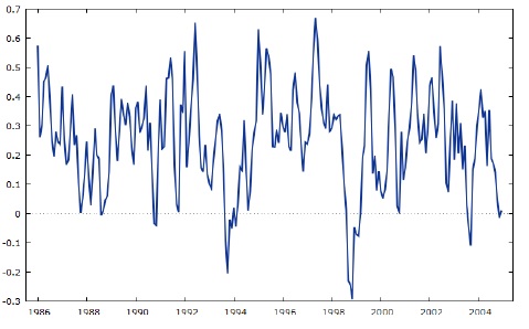 Source: Own elaboration in previous work [1]
Figure 2 shows the same time-series but for different goods. It shows an unclear pattern of co-movement between prices. Not only prices seem not be related but also, they seem to move away. In this case, the series is not stationary and thus, according with this test, we could conclude that both goods do not belong to the same market.
Figure 2: Ratio of two prices seeming not to be in the same market.
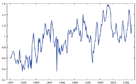 Source: Own elaboration in previous work[1]
From my point of view, for this purpose, unit root tests can be applied either with or without trend and intercept in the auxiliary regression. Initially, to test whether two goods or regions belong to the same market the trend is not relevant, since they should have a constant long-run equilibrium. In the case that the series were not stationary, repeating the test with trend would be interesting. It could explain if there exists a pattern of divergence between goods or regions. The intercept can be understood as the α coefficient exposed above. If it were zero and the test concluded stationarity, it could be a case of absolute convergence.
GRANGER CAUSALITY
Granger causality is based on the analysis of VAR models. In an easy approach, with VAR models we try to estimate the price of one good or area in function of the lags of the other price and its own lags. Granger causality analyses the null of all coefficient of the other price are zero. If the null is rejected, one price causes the other and they seem to belong to the same market.
It is possible to carry out the regressions in both ways, the first one for estimating a price and the second one for estimating the other. There could be causality in both ways but it is not a necessary requirement to conclude that there exists a causality relationship between them.
Prices displayed as the ratio of Figure 1, showed a two-way causality relationship. However, prices of Figure 2 did not show any causality relationship.
CONCLUSIONS
There are many methods to analyse if some regions or goods belong to the same relevant market. Apart from the ones exposed above, other price-based ways can be used as VEC models or PCA, and other non-price-based methods as the shock analysis or the Elzinga & Hogarty Test (1973)[10].
In general, different procedures do not use to issue contradictory answers, but they are not self-explanatory by themselves. They need to be complemented with each other to bring back the most accurate conclusion.
REFERENCES
[1] See García García, Alberto (2016). El mercado relevante: técnicas económicas y econométricas para la delimitación. Trabajo Fin de Grado. Universidad de Oviedo.
[2] Haldrup, N. (2003). “Empirical Analysis of Price Data in the Delineation of the Relevant Geographical Market in Competition Analysis. University of Aarhus, Economic Working Paper .
[3] Stigler, G. J., & Sherwin, R. A. (1985). The Extent of the Market. Journal of Law and Economics, Vol. 28, No. 3, 555-585.
[4] Granger, C. W., & Newbold, P. (1974). Spurious Regressions in Econometrics. Journal of Econometrics, 2;, 111-20.
[5] Bishop, S., & Walker, M. (1996). “Price correlation analysis: still a useful tool for relevant market definition. Lexecon.
[6] Engle, R. F. & Granger, C.W. (1987). Co-Integration and Error Correction: Representation, Estimation and Testing. Econometrica, 55(2), 251-76.
[7] Johansen, S. (1988). Statistical Analysis of Cointegration Vectors. Journal of Economic Dynamics and Control, 231-254.
[8] Alexander, Carol and Wyeth, John (1994) Cointegration and market integration: an application to the Indonesian rice market. The Journal of Development Studies, 30 (2). pp. 303-334. ISSN 0022-0388
[9] Forni, M. (2004). Using Stationarity Test in Antitrust Market Definition. American Law and Economic Review, 441-64.
[10] Elzinga, K. G., & Hogarty, T. F. (1973). The Problem of Geographic Market Definition in Antimerger Suits. Antitrust Bulletin, 18(1), pp.45-81.

 Source: Own elaboration in previous work
  Source: Own elaboration in previous work
