Could post-Brexit uncertainty have been predicted?

By Cox Bogaards, Marceline Noumoe Feze, Swasti Gupta, Mia Kim Veloso

Almost a year since the UK voted to leave the EU, uncertainty still remains elevated with the UK’s Economic Policy Index at historical highs.  With Theresa May’s snap General Election in just under two weeks, the Labour party has narrowed the gap from Conservative lead to five percentage points, which combined with weak GDP data of only 0.2 per cent growth in Q1 2017 released yesterday, has driven the pound sterling to a three-week low against the dollar. Given potentially large repurcussions of market sentiment and financial market volatility on the economy as a whole, this series of events has further emphasised the the need for policymakers to implement effective forecasting models.

In this analysis, we contribute to ongoing research by assessing whether the uncertainty in the aftermath of the UK’s vote to leave the EU could have been predicted. Using the volatility of the Pound-Euro exchange rate as a measure of risk and uncertainty, we test the performance of one-step ahead forecast models including ARCH, GARCH and rolling variance in explaining the uncertainty that ensued in the aftermath of the Brexit vote.

Introduction

The UK’s referendum on EU membership is a prime example of an event which perpetuated financial market volatility and wider uncertainty.  On 20th February 2016, UK Prime Minister David Cameron announced the official referendum date on whether Britain should remain in the EU, and it was largely seen as one of the biggest political decisions made by the British government in decades.

Assessment by HM Treasury (2016) on the immediate impacts suggested “a vote to leave would cause an immediate and profound economic shock creating instability and uncertainty”, and in a severe shock scenario could see sterling effective exchange rate index depreciate by as much as 15 percent.  This was echoed in responses to the Centre for Macroeconomics’ (CFM) survey (25th February 2016), where 93 percent of respondents agreed that the possibility of the UK leaving the EU would lead to increased volatility in financial markets and the broader economy, expressing uncertainty about the post-Brexit world.

Resonating these views, the UK’s vote to leave the EU on 23rd June 2016 indeed led to significant currency impacts including GBP devaluation and greater volatility. On 27th June 2016, the Pound Sterling fell to $1.315, reaching a 31-year low against the dollar since 1985 and below the value of the Pound’s “Black Wednesday” value in 1992 when the UK left the ERM.

In this analysis, we assess whether the uncertainty in the aftermath of the UK’s vote to leave the EU could have been predicted. Using the volatility of Pound-Euro exchange rate as a measure of risk and uncertainty, we test the performance of one-step ahead forecast models including ARCH, GARCH and rolling variance. We conduct an out-of-sample forecast based on models using daily data pre-announcement (from 1st January 2010 until 19th February 2016) and test performance against the actual data from 22nd February 2016 to 28th February 2017.

Descriptive Statistics and Dynamic Properties

As can be seen in Figure 1, the value of the Pound exhibits a general upward trend against the Euro over the majority of our sample. The series peaks at the start of 2016, and begins a sharp downtrend afterwards.  There are several noticeable movements in the exchange rate, which can be traced back to key events, and we can also comment on the volatility of exchange rate returns surrounding these events, as a proxy for the level of uncertainty, shown in Figure 2.

Figure 1: GBP/EUR Exchange Rate
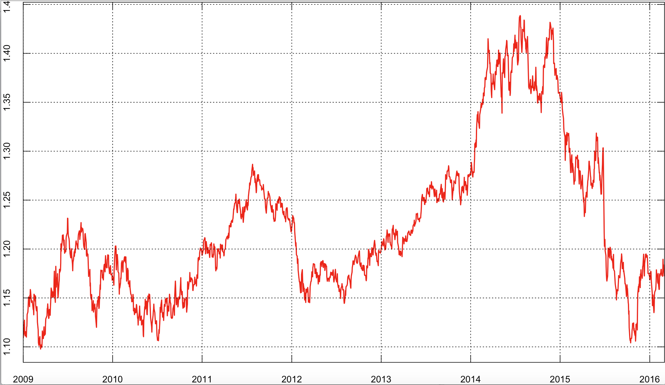
Fig 1

Source: Sveriges Riksbank and authors’ calculations

Notably, over our sample, the pound reached its lowest level against the Euro at €1.10 in March 2010, amid pressure from the European Commission on the UK government to cut spending, along with a bearish housing market in England and Wales. The Pound was still recovering from the recent financial crisis in which it was severely affected during which it almost reached parity with the Euro at €1.02 in December 2008 – its lowest recorded value since the Euro’s inception (Kollewe 2008).

However, from the second half of 2011 the Pound began rising against the Euro, as the Eurozone debt crisis began to unfold. After some fears over a new recession due to consistently weak industrial output, by July 2015 the pound hit a seven and a half year high against the Euro at 1.44.   Volatility over this period remained relatively low, except in the run up to the UK General elections in early 2015.

However, Britain’s vote to leave the EU on 23rd June 2016 raised investors’ concerns about the economic prospects of the UK. In the next 24 hours, the Pound depreciated by 1.5 per cent on the immediate news of the exit vote and by a further 5.5 per cent over the weekend that followed, causing volatility to spike to new record levels as can be seen in Figure 2.

Figure 2: Volatility of GBP/EUR Exchange Rate
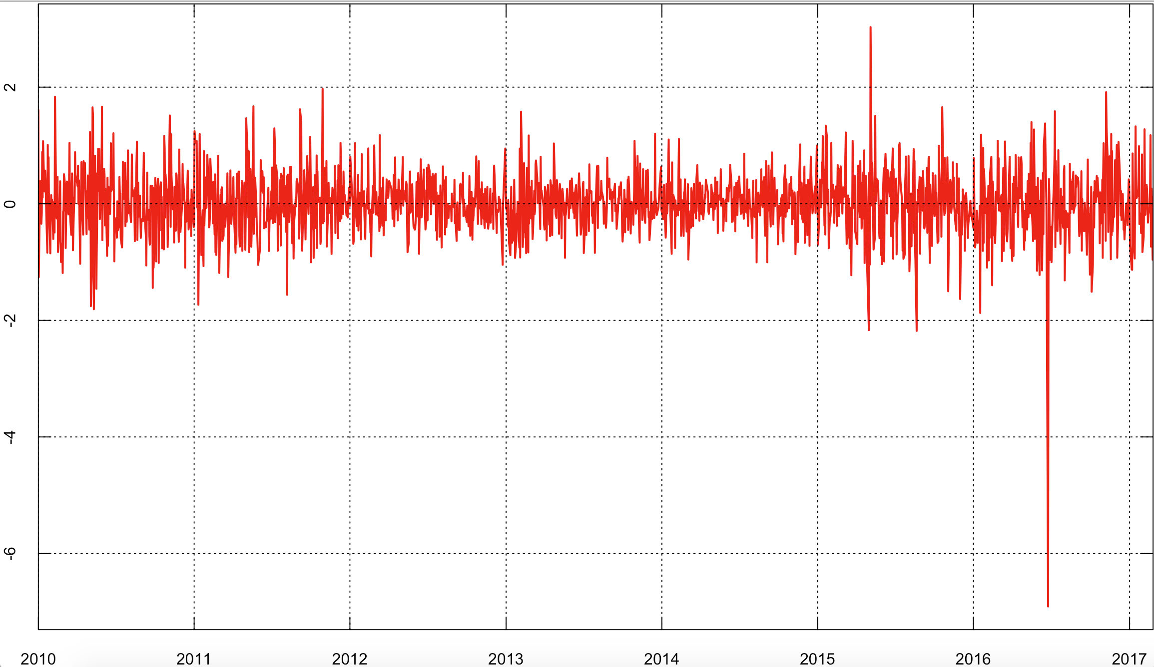
fig 2

Source: Sveriges Riksbank and authors’ calculations

As seen in Figure 1, the GBP-EUR exchange rate series is trending for majority of the sample, and this may reflect non-stationarity in which case standard asymptotic theory would be violated, resulting in infinitely persistent shocks. We conduct an Augmented Dickey Fuller test on the exchange rate and find evidence of non-stationarity, and proceed by creating daily log returns in order to de-trend the series. Table 1 summarises the first four moments of the log daily returns series, which is stationary.

Table 1: Summary Statistics

Table 1.PNG

Source: Sveriges Riksbank and authors’ calculations

The series has a mean close to zero, suggesting that on average the Pound neither appreciates or depreciates against the Euro on a daily basis. There is a slight negative skew and significant kurtosis – almost five times higher than that of the normal distribution of three – as depicted in the kernel density plot below. This suggests that the distribution of daily returns for the GBP-EUR, like many financial time series, exhibits fat tails, i.e. it exhibits a higher probability of extreme changes than the normal distribution, as would be expected.

To determine whether there is any dependence in our series, we assess the autocorrelation in the returns. Carrying out a Ljung-Box test using 22 lags, as this corresponds to a month of daily data, we cannot reject the null of no autocorrelation in the returns series, which is confirmed by an inspection of the autocorrelograms. While we find no evidence of dependence in the returns series, we find strong autocorrelations in the absolute and squared returns.

The non-significant ACF and PACF of returns, but significant ACFs of absolute and squared returns indicate that the series exhibits ARCH effects. This suggests that the variance of returns is changing over time, and there may be volatility clustering. To test this, we conduct an ARCH-LM test using four lag returns and find that the F-statistic is significant at the 0.05 level.

Estimation

For the in-sample analysis we proceed using the Box-Jenkins methodology. Given the evidence of ARCH effects and volatility clustering using an ARCH-LM test but lack of any leverage effects in line with economic theory, we proceed to estimate models which can capture this: ARCH (1), ARCH (2), and the GARCH (1,1).  Estimation of ARCH (1) suggests low persistence as captured by α1 and relatively fast mean reversion. The ARCH(2) model generates greater persistence measured by sum of α1 and α2 and but still not as large as the GARCH(1,1) model, sum of  α1 and β as shown in table 2.

Table 2: Parameter Estimates
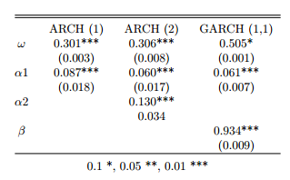
table 2

We proceed to forecast using the ARCH(1) as it has the lowest AIC and BIC in-sample, and GARCH (1,1) which has the most normally distributed residuals, no dependence in absolute levels, and the largest log-likelihood. We compare performance against a baseline 5 day rolling variance model.

Figure 3 plots the out of sample forecasts of the three models (from 22nd February 2016 to 28th February 2017). The ARCH model is able to capture the spike in volatility surrounding the referendum, however the shock does not persist. In contrast, the effect of this shock in the GARCH model fades more slowly suggesting that uncertainty persists for a longer time. However neither of the models fully capture the magnitude of the spike in volatility. This is in line with Dukich et al’s (2010) and Miletic’s (2014) findings that GARCH models are not able to adequately capture the sudden shifts in volatility associated with shocks.

Figure 3: Volatility forecasts and Squared Returns (5-day Rolling window)
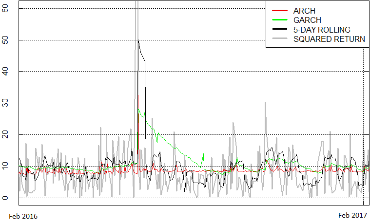
Fig 3

We use two losses traditionally used in the volatility forecasting literature namely the quasi-likelihood (QL) loss and the mean-squared error (MSE) loss. QL depends only on the multiplicative forecast error, whereas the MSE depends only on the additive forecast error. Among the two losses, QL is often more recommended as MSE has a bias that is proportional to the square of the true variance, while the bias of QL is independent of the volatility level. As shown in table 3, GARCH(1,1) has the lowest QL, while the ARCH (1) and rolling variance perform better on the MSE measure.

Table 3: QL & MSE

Table 3 QL and MSE

Table 4: Diebold- Mariano Test (w/5-day Rolling window)
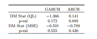
Table 4 DM test

Employing the Diebold-Mariano (DM) Test, we find that there is no significance in the DM statistics of both the QL and MSE. Neither the GARCH nor ARCH are found to perform significantly better than the 5-day Rolling Variance.

Conclusion

In this analysis, we tested various models to forecast the volatility of the Pound exchange rate against the Euro in light of the Brexit referendum. In line with Miletić (2014), we find that despite accounting for volatility clustering through ARCH effects, our models do not fully capture volatility during periods of extremely high uncertainty.

We find that the shock to the exchange rate resulted in a large but temporary swing in volatility but this did not persist as long as predicted by the GARCH model. In contrast, the ARCH model has a very low persistence, and while it captures the temporary spike in volatility well, it quickly reverts to the unconditional mean.  To the extent that we can consider exchange rate volatility as a measure of risk and uncertainty, we may have expected the outcome of Brexit to have a long term effect on uncertainty. However, we observe that the exchange rate volatility after Brexit does not seem significantly higher than before. This may suggest that either uncertainty does not persist (unlikely) or that the Pound-Euro exchange rate volatility does not capture fully the uncertainty surrounding the future of the UK outside the EU.

References

Abdalla S.Z.S (2012), “Modelling Exchange Rate Volatility using GARCH Models: Empirical Evidence from Arab Countries”, International Journal of Economics and Finance, 4(3), 216-229

Allen K.and Monaghan A. “Brexit Fallout – the Economic Impact in Six Key Charts.” www.theguardian.com. Guardian News and Media Limited, 8 Jul. 2016. Web. Accessed: March 11, 2017

Brownlees C., Engle R., and Kelly B. (2011), “A Practical Guide to Volatility Forecasting Through Calm and Storm”, The Journal of Risk, 14(2), 3-22.

Centre for Macroeconomics (2016), “Brexit and Financial Market Volatility”. Accessed: March 9, 2017.

Cox, J. (2017) “Pound sterling falls after Labour slashes Tory lead in latest election poll”, independent.co.uk. Web. Accessed May 26, 2017

Diebold F. X. (2013), “Comparing Predictive Accuracy, Twenty Years Later: A Personal Perspective on the Use and Abuse of Diebold-Mariano Tests”. Dukich J., Kim K.Y., and Lin H.H. (2010), “Modeling Exchange Rates using the GARCH Model”

HM Treasury (2016), “HM Treasury analysis: the immediate economic impact of leaving the EU”, published 23rd May 2016.

Sveriges Riksbank, “Cross Rates” www.riksbank.se. Web. Accessed 16 Feb 2017

Taylor, A. and Taylor, M. (2004), “The Purchasing Power Parity Debate”, Journal of Economic Perspectives, 18(4), 135-158.

Van Dijk, D., and Franses P.H. (2003), “Selecting a Nonlinear Time Series Model Using Weighted Tests of Equal Forecast Accuracy”, Oxford Bulletin of Economics and Statistics, 65, 727–44.

Tani, S. (2017), “Asian companies muddle through Brexit uncertainty” asia.nikkei.com. Web. Accessed: May 26, 2017

What can the risk neutral moments tell us about future returns?

Editor’s note: This post is part of a series showcasing Barcelona GSE master projects by students in the Class of 2015. The project is a required component of every master program.


Authors:
Juan Imbet, Nuria Mata

Master’s Program:
Finance

Paper Abstract:

We test if the first four moments of the risk neutral distribution implicit in options’ prices predict market returns. We estimate the risk
neutral distribution of the S&P 500 over different frequencies using a non parametric polynomial fitting, and test if the first four moments of the distribution predict returns of the S&P 500. Our results suggest that there is no evidence on this predictability power.

Presentation Slides:

[slideshare id=50497458&doc=risk-neutral-future-returns-150714070303-lva1-app6891]

The Death of Fixed Income

alumni


Alex Hansson
’13 (International Trade, Finance and Development) is an Analyst at Tribus Capital Partners in Zurich, Switzerland. Previously he was External Asset Management Analyst at Credit Suisse.


A few weeks ago I found myself sitting in the James Joyce Wine Cellar in Zurich listening to a talk by the Chief Investment Officer of one of the world’s largest asset managers’ fixed income division. Surrounded by ageing wine bottles and Swiss bankers in grey suits, the CIO put down his glass of Chateau Neuf du Pape and proclaimed, “You know, I’ve been investing in fixed income all my career, but I feel obliged to tell you that fixed income as an asset class is dead.” That was the last sentence of the speech.

Now I don’t frequent too many of these events, but ending a presentation on that kind of a bombshell was not something that I’d ever experienced before. The Swiss bankers around me shifted nervously in their seats thinking something else was coming. But the CIO did not follow up the statement with any caveats. He was undoubtedly out to provoke and had we pushed him a little he would have most likely followed up his statement with the usual spiel that one should be careful with statements like ‘this time it is different.’ He would have probably added that fixed income in terms of developed markets sovereign and corporate bonds would at some point in the future again be an interesting investment.

Nonetheless, finding out fixed income was dead was pretty exciting. Moreover, the statement was in line with a trend I had been witnessing for the past couple months whereby capital was flowing into a new asset class – alternative fixed income.

But, before moving on to this, it is worth spending a few minutes on the death of fixed income, whether temporary or not. Classic portfolio management theory will tell you to put 60% of your assets in equities (e.g. at its most basic through a S&P 500 Index ETF) and 40% in bonds (e.g. at its most basic through a Bond Index) in order to achieve diversification and lower the portfolio’s volatility. Without getting too deep into the technicalities, the thinking goes that equities outperform bonds in the long run – hence the overweight. However, bonds are included because they lower the volatility and increase the diversification of the overall portfolio. They lower the volatility because they are less risky than equities. Moreover, bonds have historically moved inversely to equities and this diversification effect has served the purpose of smoothing out the return profile of a balanced portfolio in times of market turbulence. Seeing as, nearly all investors have regular liquidity needs for, for instance, a regular mortgage payment, a smoother albeit lower return profile in the long run is more attractive than high volatility with a higher return in the very long run.

So what has changed? Norman Villamin (CIO Coutts) was recently quoted as saying that bonds used to offer an asymmetric payoff relative to equities whereas now you are left with a “symmetric asset class.” Put another way, bonds still serve the purpose of protecting capital when equities are down but no longer give you any meaningful upside. In other words by having 40% bonds you lower volatility but you no longer achieve diversification. Explaining exactly why, at least from a developed markets perspective, is not straightforward. Some analysts have highlighted that rates have been kept low to encourage lending given the slower than expected recovery in the US and Europe. Other analysts have pointed to lower inflation and central banks not feeling the pressure to increase rates. In any case, with very low returns you also have very low volatility. With low volatility even if this effect moves inversely to equities it will not be ‘strong enough’ to provide the desired counterbalancing effect. Think of two grown men on a seesaw where one gets replaced by a child, no matter how much the child jumps up and down on the plank, they will not significantly propel the man into the air. Whatever the reasons for this phenomenon, most seem to agree that a low rate environment will be the norm for some time to come.

Many investors realize that if rates remain low it will become more difficult to find bonds yielding attractive returns without taking on excessive risk. In terms of fixed income this generally means looking towards emerging market debt or distressed corporate bonds. To be clear some investors have successfully gone down this route, such as, Michael Hasenstab (CIO Franklin Templeton) who has became famous for his bullish speeches on Ukrainian debt. Nonetheless this dynamic has led to many investors leaving fixed income in favor of equities. That trend is clearly reflected by the fact that the largest fund by assets under management has over the last year shifted from the PIMCO Total Return fund (a fixed income product) to the Vanguard Total Stock Market Index (an equity product). The leaving of Mr. Gross from PIMCO no doubt also contributed to this shift.

With the recent prolonged bull market most investors have shut their eyes to the increased volatility and enjoyed the attractive returns they have seen from their portfolios. However, some sophisticated investors have elected not to move their fixed income exposure to equities. Some have chosen to put assets into well-known alternatives like private equity or real estate. But these asset classes do not offer the same advantages that fixed income did.

As outlined above fixed income was liked because, first, it was relatively low risk. Second, it paid a steady regular coupon, which was liked not just by private investors but especially pension and insurance funds, which have regular liquidity needs. Third, it paid a handsome return of anywhere from 5.00% to 8.00% (historically seen). To put that into perspective, a ten year German Government Bond pays you less than 1.00% currently. A private equity or real estate investment conversely can mean having to lock up capital for ten years, with no regular coupon payment, and with no guarantee for handsome reward.

Given this, many of these sophisticated investors have turned to a different asset class that has emerged largely as a product of new lending opportunities. It is often referred to as Alternative Fixed Income. These opportunities have to a large extent emerged as a product of new banking regulations. Simply put, banks have been forced to move away from certain types of lending and new non-bank credit providers have stepped in to fill this void offering new investment opportunities. Indeed, according to Alliance Bernstein, since 1980 the nonfinancial corporate and mortgage credit outstanding has grown by ca. USD 18.9tn whereof USD 15.0tn can be attributed to non-banks.

This trend of lending by non-banks has been accelerated largely as a product of post-crisis regulation. In Europe, the most important regulation framework for this trend has been Basel III. This framework stipulated that banks now have much higher capital requirements as well as having to take on higher operational costs for certain types of lending. This has been most pronounced for investments with longer investments horizons, which therefore cannot match bank-liability structures subject to daily liquidity requirements.

There are literally hundreds of structures that have emerged to take advantage of this systemic shift. The biggest opportunities for alternative credit providers have been in corporate loans, commercial real estate loans, residential real estate loans, and infrastructure loans. Many new organizations have been set up and are raising capital from investors in order to lend to corporations and real estate developers in the same way banks used to. The lenders pay a coupon on the loan, the new firms take a cut, and the investor gets a regular coupon payment at a tolerable risk and a much higher return than they would have in traditional fixed income.

This systemic shift has created opportunities along the entire supply chain of lending. It stretches from the most logical to the most niche areas you can think of, and no doubt this is just the beginning. Below I will give two examples of the most common constellations.

Most commonly you see new organizations made up of former bankers. They leave or are made redundant by their employer. They take with them an intimate knowledge of that bank’s loan book as well as the skillset to analyze other banks’ loan books. They then raise capital in a fund structure (funded by our sophisticated investors above) and begin buying loans from banks that can no longer be kept on their balance sheets. This can take many different forms. The easiest is a pure purchase at a discount where the new organization takes over the loan. Typically this happens via a Collateralized Loan Obligation (CLO) which is a securitized asset backed by a pool of debt. Another variety is a situation where banks have debt on their balance sheet which is highly attractive from a return perspective but which they cannot keep on their balance sheet. They therefore use something called Regulatory Capital Relief Trades (CRTs) in order to temporarily transfer risky assets off their balance sheets to one of these new organizations which in turn charge interest on the assets while on their balance sheets. Finally you have situations where the bank will give an organization access to their pipeline of loan opportunities. This setup is rarer and requires a very close relationship between the bank and the new organization. Essentially, these new organization can sift through bank’s pipeline of lending opportunities and chose to take on any loans they find attractive. In return the bank receives a share of the profits.

The other more common constellation of new organizations is direct loans that banks used to be able to do. Indeed, many of these organizations are whole teams that used to do the same thing at their former employers. A great example is Renshaw Bay. Renshaw Bay was setup by the former co-CEO of J.P. Morgan’s Investment Bank – Bill Winters. The firm runs a real estate strategy that is “focused on direct, whole loan origination of commercial real estate loans… and seeks to take advantage of the lack of financing available to real estate borrowers”. They also run a structural finance strategy, which looks to “capitalize on opportunities driven by regulatory change and the retreat of capital.” There are now new organizations (or old organizations which have seen a significant uptick in demand) that are doing the same thing in corporate loans, real estate loans, infrastructure loans, or even leverage loans to private equity firms.

It is still relatively early days and no one yet completely understands the full implications of this systemic shift. Perhaps the setup is better, seeing as you have more specialized niche players, often with much of their internal capital at risk, and unhindered by bureaucracy associated with banks running these new organizations. Or perhaps this setup is riskier, since at the same time you also have small, inexperienced, and at times highly leveraged organizations with less oversight then banks used to have. Added to this increasing numbers of pension funds and insurance companies are investing in these structures. Undoubtedly there will be some financial cowboys who have cut corners in order to have first mover advantage. At the same time you will undoubtedly have a lot of smart people who will make themselves and their investors a lot of money. Clearly, it is going to be very interesting to monitor these developments to see whether this shift turns out to be a good one or a bad one.